Time-series Data: The Pulse of the Digital Era

✍️By Thanh Ho

•

📅May 21, 2026

In the digital era, data no longer exists merely as static snapshots. Everything around us is constantly moving and evolving over time. From a patient's heart rate and atmospheric temperatures to the second-by-second fluctuations of the stock market – all are recorded as Time-series Data. For anyone stepping into the fields of Data Science, Artificial Intelligence (AI), or Quantitative Finance/Investing, a solid understanding of Time-series data is an essential stepping stone. This article will help you approach this unique data type, from the most intuitive concepts to advanced processing techniques used in practice.

1. What is Time-series Data?

Time-series Data is a collection of observations (metrics, measurements) of the same entity recorded sequentially at equally spaced time intervals.

A standard Time-series data point always consists of two core components:

Timestamp: Serves as the positioning coordinate (e.g., 2026-05-19 09:00:00).
Value: The technical metric measured at that specific timestamp (e.g., stock price, temperature, CPU usage).

Distinguishing Time-series from Other Data Structures

To understand this better, let's compare Time-series with two other common data structures:

Cross-sectional Data: A snapshot of multiple subjects at a single point in time.
- Example: The revenue of 100 tech companies on December 31, 2025.
Panel Data (Longitudinal Data): A combination of both worlds – tracking multiple subjects across multiple time periods.
- Example: The revenue of 100 tech companies recorded continuously from 2020 to 2025.
Time-series Data: Focuses strictly on tracking a single subject over multiple consecutive time periods.
- Example: The daily stock price fluctuations of a single corporation.

2. Unique Characteristics of Time-series Data

Unlike tabular data where rows are assumed to be independent, Time-series data carries its own distinct characteristics:

2.1. Temporal Dependency

In traditional statistics, a key assumption is that observations must be Independent and Identically Distributed (I.I.D). However, Time-series completely violates this assumption. Today's value ( $Y_{t}$ ) is heavily influenced by yesterday's value ( $Y_{t - 1}$ ) and preceding days. This phenomenon is known as Autocorrelation.

2.2. Non-stationarity

Real-world data often changes its behavior over time. The Mean and Variance of the series are not constant but fluctuate continuously (e.g., a nation's GDP tends to grow steadily over decades). This "non-stationary" nature poses a major challenge for traditional forecasting models, which typically require data to be stationary.

2.3. Temporal Resolution

Data can be collected at various frequencies: every millisecond (high-frequency algorithmic trading), hourly (weather temperature), monthly (Consumer Price Index - CPI), or annually. Synchronizing data frequency is a critical step in time-series analysis.

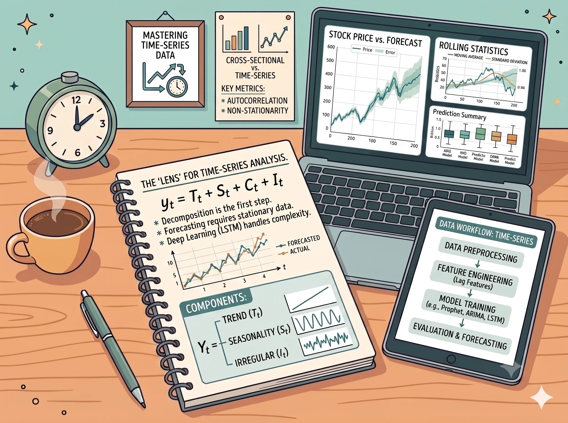
3. Core Components of Time-series Data

A complex time-series is usually a blend of four fundamental components:

                  ┌───────────────────────────────┐
                  │    Time-series Data (Y_t)     │
                  └───────────────┬───────────────┘
         ┌────────────────────────┼────────────────────────┐
┌────────┴────────┐      ┌────────┴────────┐      ┌────────┴────────┐
│     Trend       │      │   Seasonality   │      │    Cyclical     │
└─────────────────┘      └─────────────────┘      └─────────────────┘
                                  │
                         ┌────────┴────────┐
                         │  Irregular/Noise│
                         └─────────────────┘

Trend ( $T_{t}$ ): The long-term direction of the data (upward, downward, or sideways) over a prolonged period.
- Example: The global population aging trend or the growth rate of internet users.
Seasonality ( $S_{t}$ ): Fluctuations that repeat at fixed, short-term intervals (usually under a year) due to calendar, weather, or cultural factors.
- Example: Electricity consumption spiking in the summer, or retail sales peaking during the holiday season.
Cyclical ( $C_{t}$ ): Upward or downward swings that do not have a fixed period and typically last for several years, heavily influenced by macroeconomic or business cycles.
- Example: Central bank monetary tightening/easing cycles, or real estate market freeze periods.
Irregular/Noise ( $I_{t}$ ): Unpredictable fluctuations caused by random events, natural disasters, or market shocks.
- Example: The severe downturn in the global aviation industry when the COVID-19 pandemic hit in early 2020.

Two Basic Mathematical Decomposition Models

To analyze these components, data scientists typically utilize two mathematical forms:

Additive Model: Applied when the amplitude of seasonal fluctuations does not change with the trend.

$Y_{t} = T_{t} + S_{t} + C_{t} + I_{t}$

Multiplicative Model: Applied when the amplitude of seasonal fluctuations increases or decreases in proportion to the trend.

$Y_{t} = T_{t} \times S_{t} \times C_{t} \times I_{t}$

4. Real-World Applications of Time-series Data

Time-series data is omnipresent across most critical sectors of life:

Finance and Investment: Second-by-second price fluctuations (Tick data) of Forex pairs, stocks, or Crypto. Quarterly/annual financial reports are also archived to analyze long-term trends for corporate valuation.
System Operations & IT (DevOps): VPS monitoring systems plot continuous metrics (such as % CPU Usage, RAM consumption, and Bandwidth) to trigger automated incident alerts.
Healthcare & Medicine: Electrocardiograms (ECG) or Electroencephalograms (EEG) record real-time electrical signals of the heart/brain for early detection of stroke pathologies.
Meteorology & Environment: Hourly PM2.5 fine dust indexes for air quality warnings, or cumulative monthly rainfall to forecast droughts.

5. Core Techniques for Working with Time-series Data

Working with time-series requires a completely different toolkit and mindset compared to standard tabular data. Here is the standard technical workflow:

5.1. Data Preprocessing

Handling Missing Data (Imputation): You cannot use standard mean imputation, as it breaks temporal continuity. Instead, use:
- Forward Fill: Carries the last known value forward into the missing slot.
- Linear Interpolation: Estimates missing values linearly based on the closest neighboring points.
Resampling:
- Downsampling: Decreasing data frequency—e.g., aggregating seconds into hours (using mean or sum).
- Upsampling: Increasing data frequency—e.g., expanding daily data to hourly intervals (combining interpolation methods to smooth the curve).

5.2. Feature Engineering

Lag Features: Creating new variables based on historical values. For instance, to forecast today's housing price, we introduce "yesterday's price" ( $Y_{t - 1}$ ) and "the price from a week ago" ( $Y_{t - 7}$ ) as features into the model.
Rolling Statistics: Computing statistical metrics within a moving time window, such as a 30-day Moving Average.

5.3. Analysis and Forecasting Models

Classical Statistical Models:
- ARIMA (AutoRegressive Integrated Moving Average): Combines autoregression, differencing (to achieve stationarity), and a moving average of residual errors.
- Exponential Smoothing (Holt-Winters): A powerful smoothing model designed for data with strong seasonal patterns.
Advanced Machine Learning & Deep Learning:
- Prophet: An open-source model developed by Meta, highly efficient at handling data with multiple seasonalities (weekly, yearly) and holiday effects.
- Deep Learning (LSTM, GRU, Transformer): Neural network architectures capable of retaining long-term dependencies, perfect for highly complex non-linear time series like financial behavior or natural language processing.

6. Dangerous Pitfalls to Avoid

When starting out with Time-series data, many data engineers fall into serious logical traps, resulting in models that look "picture-perfect" during validation but "completely collapse" in production (out-of-sample).

6.1. Data Leakage in Cross-Validation

In static datasets, we commonly use K-Fold Cross-Validation (randomly shuffling data into training and testing sets). Never apply this to Time-series data!

If you shuffle time-series data randomly, your model will use future information (e.g., May 20th) to predict the past (e.g., May 19th). This leads to severely biased and overly optimistic evaluation results.

Solution: Use Time Series Split (Walk-Forward Validation). Training must strictly use data that occurred before the time point being predicted.

Training (Past)       ──► Testing (Future)
[ May 19 ]            ──► [ May 20 ]           (Valid)
[ May 19 & May 20 ]   ──► [ May 21 ]           (Valid)

6.2. Look-ahead Bias

This error occurs when calculating a feature at time $t$ , but you accidentally incorporate information that only becomes available at time $t + 1$ .

Example: Using today's closing price to decide an entry order early this morning. Always rigorously verify whether a feature was actually available at the exact moment the decision had to be made.

6.3. Spurious Correlation

Two entirely unrelated datasets can show an incredibly strong statistical correlation simply because they both trend upward over time.

Classic Example: A chart showing that both ice cream sales and forest fires spike in July. In reality, both are driven by a third confounding factor: "hot summer weather."

Solution: Apply Differencing (the difference between consecutive data points) to eliminate the underlying trend before analyzing correlations.

Conclusion

Time-series data is a dynamic canvas, where every data point is a piece of history that helps us engineer forecasts for the future. Mastering the time-series mindset not only empowers you to build smarter AI systems but also serves as a sharp weapon to optimize quantitative financial investment decisions with high efficiency.